[Tutorial] How to measure mass flow rate using PhysLoad

[umar.techboy]

In case we have a changing mass, for example,

1. a leaking faucet
2. an evaporating liquid,
3. a powder being poured,

or a similar situation, the rate of change of mass can be measured using PhysLoad.

Here is what needs to be done:

1. Attach PhysLoad
2. Create a low pass filter (optional but recommended)
3. Differentiate

For a fresh PhysLogger session, just follow the screenshots and start measuring. An improvised subset of the same steps can be used to integrate flow rate into an existing session too.

1. Connect PhysLogger if not already done.
   

   

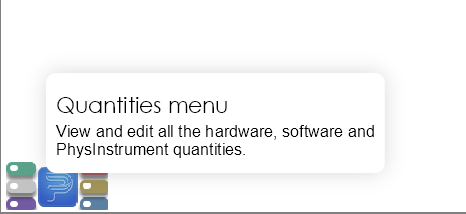
2. Open the quantities menu:
   

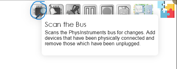
3. Make sure you see a PhysLoad in the quantities menu. If you don’t, make sure you have connected a PhysLoad to one of the digital channels of PhysLogger and rescan the PhysInstruments bus to detect it:
   

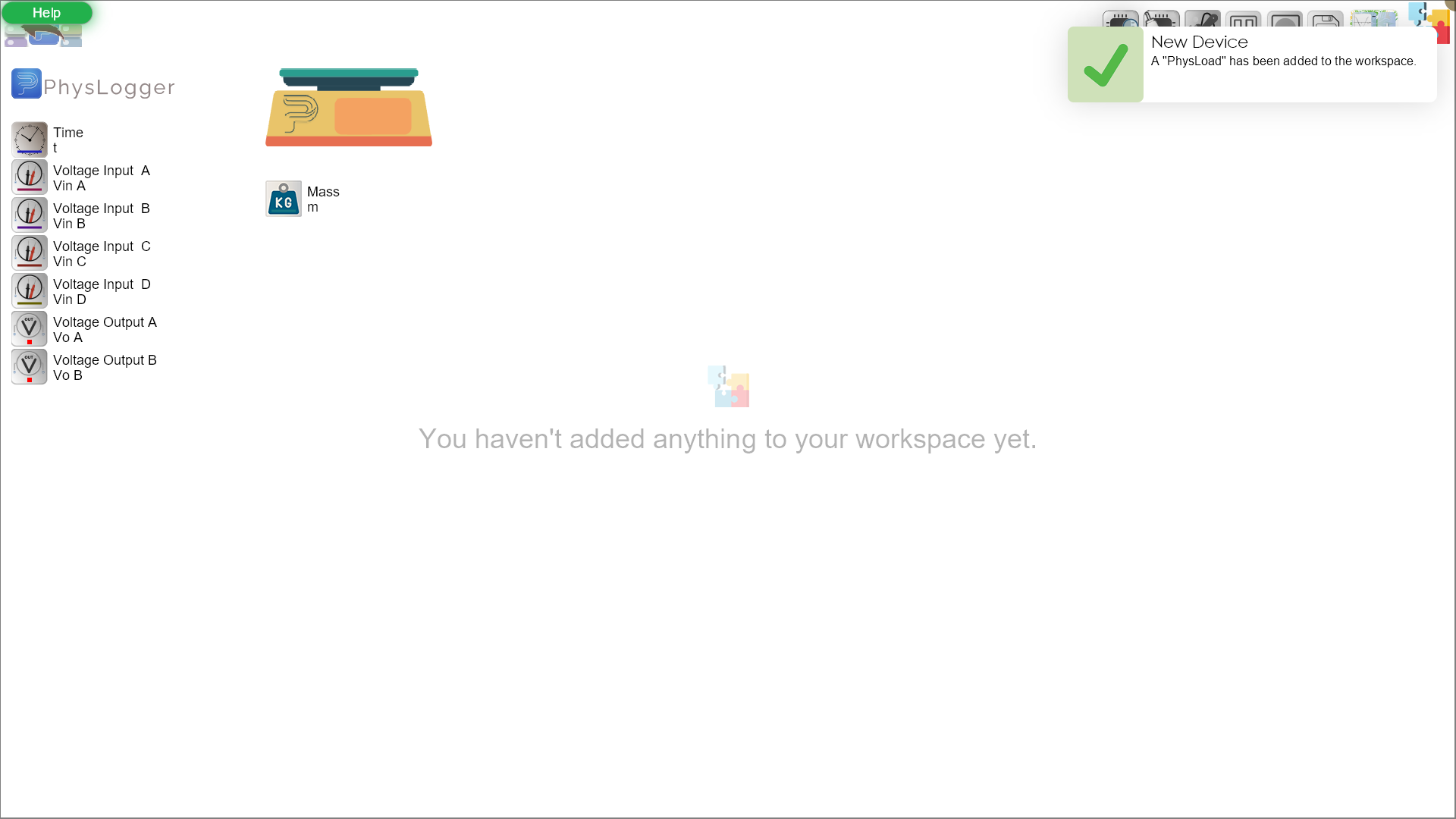
4. Once done, you should see a PhysLoad quantity in the quantities menu. Even if you don’t try a different USB cable to connect PhysLogger to PhysLoad, try a different digital port and hit the “Scan the Bus” button again.
   

   

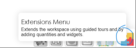
5. Go to the extensions menu now:
   

6. Choose the wizard:
   

   

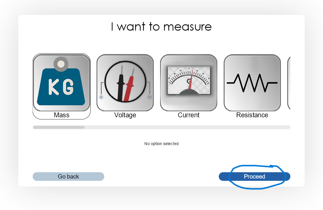
7. Go to Measure:
   

   

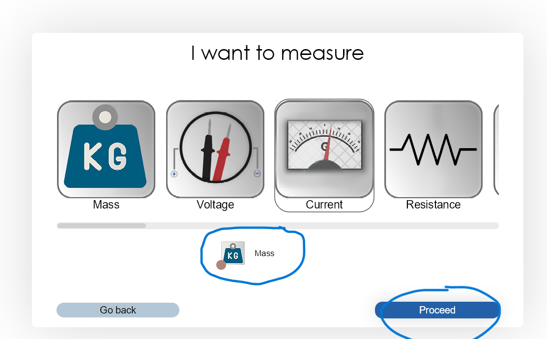
8. PhysLoad should appear here now as “Mass” quantity. In case multiple PhysLoads are connected, they all show up here as “Mass” along with other quantities that originate from other digital quantities.
   

   

9. On selection, the quantity is configured and added to the wizars stack. Hit “Proceed” to add setup further:
   

   

10. Choose to create a new live plot. If you don’t create one, you will have to manually add the quantity to another plot.
    

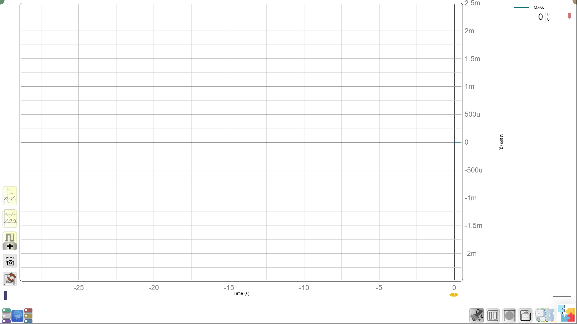
11. Once dropped, the plot should start displaying the mass. You can touch the load plate of PhysLoad to verify that it is in action. In the attached screenshot, you are observing a constant “0” mass, it is because in this example, a virtual PhysLoad is connected just to demonstrate the process. Yours might show a lot of noise in the range of 2-5g.

@forumAdmin

See PhysLoad Features for more details

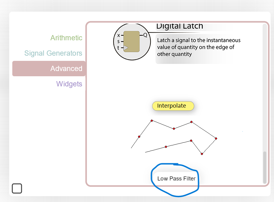
12. We now need to add a filter and a differentiation quantity. For that, once again, open the “Extensions Menu” and select “Build from Scratch” this time:
    

    

13. First, choose the Low-pass filter (or simple Filter) quantity from “Advanced” quantities. You can work without a low pass but not without expecting a lot of noise in the differentiated quantity.
    
    

    

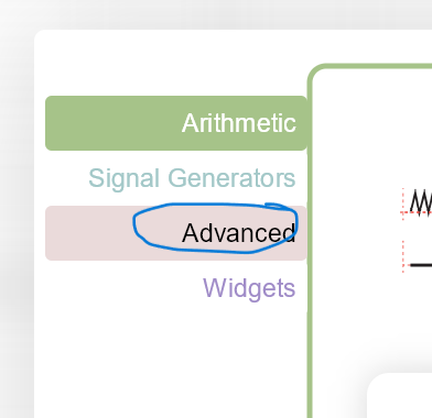
14. Tell the source quantity, the quantity that we want to filter. It is our mass quantity.
    
    

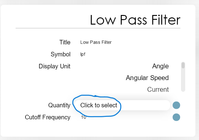
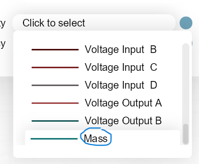
You might also want to rename the filter to something like “Filtered mass” or more elegantly, “$$m_filtered” or “$m_filtered$”. Putting a “$$” pair at the beginning or “$” around a name or a symbol will make PhysLogger interpret the text as a Latex (well, as close to latex as possible).

15. Finally add a differentiation from the same “Advanced” menu. This time, make differentiate the filter quantity (or mass quantity, in case you skipped the filter in previous steps). You might want to rename this quantity too. something like “$$\Delta m/\Delta t” or “$$\delta m/\delta t” should suite this quantity.

16. You are almost done. All you now need to do is to add another plot in our LivePlot and drop the newly created quantity on to an available axis that is highlighted by a blue region.
    
    

    

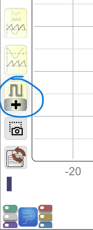
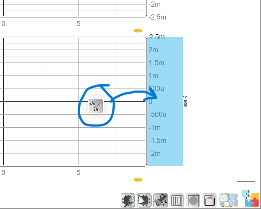
Viola! You are all done.